Lambda caluclus 是一种描述语言机制的 core language。除此之外,还有其他 calculi:
- pi-calculus: a popular core language for defining the semantics of message-based concurrent languages
- object calculus: distills the core features of object-oriented languages
传统的 Lambda Calculus 是一个 core language,可以给它添加其他特性构成新的语言。
- the pure untyped lambda-calculus:λ
- the lambda-calculus extended with booleans and arithmetic operations:λNB
Basics
在 λ 演算中一切都是函数,包括函数的输入值和返回值都可以用函数表示。
λ 演算的中的 term 指的是任意的 term,而其中以 λ 开头的 term 被称为 lambda-abstractions。
在 λ 演算中,其语法由三种形式组成:
- 变量:
x - 抽象:一个 term
t中抽象出一个变量x,记作 \(\lambda x.t\) - 应用:将一个 term
t2作为参数传入另一个 termt1,记作t1 t2
\begin{aligned} t \Coloneqq & & (\text{terms}) \\ & x & (\text{variable}) \\ & \lambda x.t & (\text{abstraction}) \\ & t\ t & (\text{application}) \\ \end{aligned}
Abstract and Concrete Syntax
编程语言的语法有两种方式可以表示:一种是通常看到的字符串形式的代码,称为 concrete syntax(surface syntax);另一种是编译器或者解释器中用树结构(AST)表示的语法,称为 abstract syntax。后者有利于对代码的结构进行操作,因此常在编译器和解释器中使用。
将 concrete syntax 转换为 abstract syntax 的过程共分为两步:
- 通过 lexer 将字符串解析成一个 token 序列,token 表示最小的语法单元,删除空格、注释等内容,并进行简单的转换(如数字数制、字符串等)
- 通过 parser 将 token 序列转换成 AST,这个阶段要处理运算符的结合性等问题
除此之外,一些语言还有其他的解析过程。例如将语言的一些特性定义成更基本的特性的 derived forms。然后定义 internal language(IL)表示一门仅包含了必要的 derived forms 的 core language,同时定义 external language(EL)表示包含了所有 derived forms 的 full language。并且在 parse 的阶段后,将 EL 转换成 IL,从而使得语言的核心更简单。
为了减少冗余括号,本书书写 λ 表达式时会遵从两个规则:
- application 采用左结合,即
s t u表示(s t) u - abstraction 的 body 部分尽可能得长,如 \(\lambda x. \lambda y. x y x\) 表示 \((\lambda x. (\lambda y. (x y) x))\)
Variables and Metavariables
出于习惯,t 表示任意的 term,xyz 表示任意的 metavariables。
Scope
当变量 x 出现在 abstraction \(\lambda x.t\) 的 body 部分时,称其是被约束的(bound),\(\lambda x\) 被称为 binder。反之,如果变量不被约束,在称为是自由的(free)。例如 \((\lambda x.x)x\) 中第一次出现的 x 表示一个 binder,第二次出现的 x 是 bound 的,第三次出现的 x 是 free 的。
如果一个 term 没有自由变量,则称为封闭的(closed)。封闭的 term 又被称为组合子(combinators),例如 identify function:
\[ \mathtt{id} = \lambda x.x; \]
Static-scoping and Dynamic-scoping
在编程语言中,scope 一般分为 static-scoping 和 dynamic-scoping:
- 在 static-scoping 中,一个变量的作用域是由它在源代码中的位置决定的。因此编译器或解释器可以仅通过分析代码结构(而不是实际执行代码)来确定变量的作用域。
- 与之相对的是 dynamic-scoping,变量的作用域由程序的运行时调用顺序决定。
下面是一个例子:
let x = 10 in
  let f = (lambda y. x + y) in
    let x = 20 in
      f 5
在 static-scoping 中,这个表达式的值是 15,因为 f 的作用域是整个 let 表达式,所以 f 中的 x 是第一个 x,而不是第二个;而在 dynamic-scoping 中,这个表达式的值是 25,因为 f 中的 x 是第二个 x。
Operational Semantics
在 pure lambda calculus 中不包含任何数字、运算符等,唯一的运算只有 application。
Application 的步骤为将左侧的 abstraction 中的约束变量替换成右侧的组件。记作
\[ (\lambda x.t_{12}) t_2 \rightarrow [x \mapsto t_2] t_{12} \]
其中 \([x \mapsto t_2] t_{12}\) 表示将 \(t_{12}\) 中所有的自由出现的 \(x\) 替换成 \(t_2\)。例如 \((\lambda x.x) = y\),\((\lambda x.x(\lambda x.x))(u r) => u r (λx.x)\)。
类似于 \((\lambda x.t_{12}) t_2\) 的表达式被称为 redex(reducible expressions)。Redex 可以用 beta-reduction 进行重写。
Evaluation strategies
例子:
\[ (\lambda x.x)\ ((\lambda x. x))\ (\lambda z. (\lambda x.x))\ z)) = \mathtt{id}\ (\mathtt{id}\ (\lambda z. \mathtt{id}\ z)) \]
Full beta-reduction:随便选一个 redex 进行 reduce
\begin{aligned} & \mathtt{id}\ (\mathtt{id}\ (\lambda z. \underline{\mathtt{id}\ z})) \\ \rightarrow {}& \mathtt{id}\ (\underline{\mathtt{id}\ (\lambda z. z)}) \\ \rightarrow {}& \mathtt{id}\ (\lambda z.z) \\ \rightarrow {}& \lambda z.z \end{aligned}
由 Church-Rosser property,λ 演算在 full beta-reduction 下是 confluent 的。(求值顺序不影响结果)
Normal order strategy:先 reduce 最外面、最左边的 redex
\begin{aligned} & \underline{\mathtt{id}\ (\mathtt{id}\ (\lambda z. \mathtt{id}\ z))} \\ \rightarrow {}& \underline{\mathtt{id}\ (\lambda z. \mathtt{id}\ z)} \\ \rightarrow {}& \lambda z.\ \underline{\mathtt{id}\ z} \\ \rightarrow {}& \lambda z.z \end{aligned}
Call by name strategy:call by name 和 normal order strategy 类似,但是它不允许在 abstraction 内部进行 reduces
Call by name 在调用的时候不计算值,而是直接传入对应的位置,用到的时候再调用
\begin{aligned} & \underline{\mathtt{id}\ (\mathtt{id}\ (\lambda z. \mathtt{id}\ z))} \\ \rightarrow {}& \underline{\mathtt{id}\ (\lambda z. \mathtt{id}\ z)} \\ \rightarrow {}& \lambda z.\ \underline{\mathtt{id}\ z} \\ \end{aligned}
Call-by-name 被很多语言都实现了,比如 Algol60 和 Haskell。其中 Haskell 的更加特殊,使用了一个优化过的形式 call by need:在第一次求值后会记录下结果,后面进行复用,这是因为 Haskell 的 pure 的。
Call by value strategy (Applicative-order):最常用的 redex 策略。reduce 外层,且一个 redex 会被 reduce 仅当它的参数已经是一个 value。value 即一个不能被 reduce 的形式,包括 lambda abstractions,numbers,booleans 等。
\begin{aligned} & \mathtt{id}\ \underline{(\mathtt{id}\ (\lambda z. \mathtt{id}\ z))} \\ \rightarrow {}& \underline{\mathtt{id}\ (\lambda z. \mathtt{id}\ z)} \\ \rightarrow {}& \lambda z.\ \underline{\mathtt{id}\ z} \\ \end{aligned}
其中,normal order strategy 和 call by name 都是 partial evaluation。它们在 reduce 的时候可能函数还没有被 apply。
Call by value 是 strict 的,即无论参数有没有用到,都会被 evaluate;反之 call by name 和 call by need 则只有在用到某个参数的时候才计算。
本书后面都使用 call by value。因为这样实现 exceptions 和 reference 会更简单。
Programming in the Lambda-Calculus
Multiple Arguments
λ 演算中的多参数函数是通过高阶函数(higher-order functions)实现的。
假设 \(s\) 是一个包含自由变量 x、y 的 term,f 是一个参数为 x、y 的函数:
\[ f = \lambda x. \lambda y. s \]
\begin{aligned} f v w & = (f\ v) w \\ & \rightarrow (\lambda y.[x \mapsto v]s)\ w \\ & \rightarrow [y \mapsto w][x \mapsto v]s \end{aligned}
这种参数一个个被 apply 的过程称为 currying。
Church Boolean
λ 演算中的 boolean 也可以用 λ 表达式表示。其中 true 和 false 分别是一个接受两个参数的函数,true 返回第一个参数,false 返回第二个参数。这种表示可以看作是 testing the truth of a boolean value。
\begin{aligned} \mathtt{tru} &= \lambda t. \lambda f. t; \\ \mathtt{fls} &= \lambda t. \lambda f. f; \end{aligned}
下面定义一个类似 if 的 combinator test。在 test b v w 中,当 b 为 true 时返回 v,反之返回 w。
\[ \mathtt{test} = \lambda l. \lambda m. \lambda n. l\ m\ n; \]
\begin{aligned} &\mathtt{test}\ \mathtt{tru}\ v\ w \\ = {}& \underline{(\lambda l. \lambda m. \lambda n. l\ m\ n)\ \mathtt{tru}}\ v\ w \\ \rightarrow {}& \underline{(\lambda m. \lambda n. \mathtt{tru}\ m\ n)\ v}\ w \\ \rightarrow {}& \underline{(\lambda n. \mathtt{tru}\ v\ n)}\ w \\ \rightarrow {}& \mathtt{tru}\ v\ w \\ = {}& \underline{(\lambda t. \lambda f. t)\ v}\ w \\ \rightarrow {}& \underline{(\lambda f. v)\ w} \\ \rightarrow {}& v \end{aligned}
类似的,还可以定义 booleans 相关的逻辑运算:
and:如果第一个数是tru,则看第二个数;否则直接返回fls\begin{alignat*}{2} &\mathtt{and} && = \lambda b.\lambda c.b\ c\ \mathtt{fls}; \\ &\mathtt{and2} && = \lambda b.\lambda c.b\ c\ b; \end{alignat*}
or:如果第一个数是tru,则返回tru;否则看第二个数\begin{alignat*}{2} &\mathtt{or} &&= \lambda b.\lambda c.b\ \mathtt{tru}\ c; \\ &\mathtt{or2} &&= \lambda b.\lambda c.b\ b\ c; \end{alignat*}
not:\[ \mathtt{not} = \lambda b.b\ \mathtt{fls}\ \mathtt{tru} \]
示例:
\begin{aligned} & \mathtt{and}\ \mathtt{tru}\ \mathtt{tru} \\ = {}& \underline{(\lambda b. \lambda c.b\ c\ \mathtt{fls})\ \mathtt{tru}\ \mathtt{tru}} \\ \rightarrow^* & \mathtt{tru}\ \mathtt{tru}\ \mathtt{fls} \\ = {}& \underline{(\lambda t. \lambda f.t)\ \mathtt{tru}\ \mathtt{fls}} \\ \rightarrow^* & \mathtt{tru} \end{aligned}
Pair
\begin{alignat*}{2} &\mathtt{pair} &&= \lambda f. \lambda s. \lambda b.b\ f\ s; \\ &\mathtt{fst} &&= \lambda p.p\ \mathtt{tru}; \\ &\mathtt{snd} &&= \lambda p.p\ \mathtt{fls}; \end{alignat*}
示例:
\begin{aligned} &\mathtt{fst}\ (\mathtt{pair}\ v\ w) \\ = {}& \mathtt{fst}\ (\lambda b.b\ v\ w) \\ = {}& (\lambda p.\ p\ \mathtt{tru})(\lambda b.b\ v\ w) \\ \rightarrow {}& (\lambda b.b\ v\ w)\ \mathtt{tru} \\ \rightarrow {}& \mathtt{tru}\ v\ w \\ \rightarrow^* & v \end{aligned}
Church Numerals
λ 演算中,自然数用 combinator 表示。其中,s 和 z 分别代表 succ 和 zero。 其意义为递归对于 z 调用 n 次 s,即 \(s^n(z)\)。(The number n is represented by a function that does something n times)
个人感觉在 λ 演算中,对于数据强调的不是如何存储,而是如何去使用它们。所以
tru和fls对应了程序的选择结构;自然数对应了程序的归纳结构(类似于循环)。
\begin{aligned} \mathrm{c}_{0} &= \lambda s.\lambda z.\mathrm{z}; \\ \mathrm{c}_{1} &= \lambda s.\lambda z.\mathrm{s}\ \mathrm{z}; \\ \mathrm{c}_{2} &= \lambda s.\lambda z.\mathrm{s}\ (\mathrm{s}\ \mathrm{z}); \\ \mathrm{c}_{3} &= \lambda s.\lambda z.\mathrm{s}\ (\mathrm{s}\ (\mathrm{s} \mathrm{z})); \end{aligned}
不难发现,\(C_0\) 和 \(\mathtt{fls}\) 的表示形式相同!
求后继数:直接套上一层
s(由于是 currying 的形式,所以结果还是 \(\lambda s.\lambda z.t\))\begin{alignat*}{2} & \mathtt{scc} &&= \lambda n.\lambda s.\lambda z.s\ (n\ s\ z); \\ & \mathtt{scc2} &&= \lambda n.\lambda s.\lambda z.\ n\ s\ (s\ z); \end{alignat*}
求和:
m的s不变,z变成n,意为在n上应用m次,即 \(s^{n+m}(z) = s^n(s^m(z))\)\[ \mathtt{plus} = \lambda m.\lambda n.\lambda s.\lambda z. m\ s\ (n\ s\ z); \]
乘法:第一个数字的
s变成plus n,意为在z上调用m次plus n,即 \(s^{nm}(z) = (s^n)^m(z)\)\begin{alignat*}{2} & \mathtt{times} &&= \lambda m.\lambda n.m\ (\mathtt{plus}\ n)\ c_0; \\ & \mathtt{times2} &&= \lambda m.\lambda n.\lambda s.\lambda z.\lambda.m\ (n\ s)\ z; \\ & \mathtt{times3} &&= \lambda m.\lambda n.\lambda s.m\ (n\ s); \end{alignat*}
其中
times2比较有意思。其中n s的基数部分(z)接受的是上一次加法的结果,这样调用m次,即执行m次加法。times3是times2的化简形式。幂次:
\begin{alignat*}{2} & \mathtt{power} &&= \lambda m.\lambda n.\lambda s.n\ (\mathtt{times}\ m)\ c_1; \\ & \mathtt{power2} &&= \lambda m.\lambda n.\lambda s.\lambda z.n\ (\lambda f.m\ f\ s)\ s\ z; \\ & \mathtt{power3} &&= \lambda m.\lambda n.n\ m; \end{alignat*}
其中有意思的是
power2,可以从power化简,也可以这么理解:考虑现在已经有了
\begin{aligned} g_i &= \lambda f’. \lambda z.\underbrace{f’ (f’ ( \cdots f’ (z) \cdots ))}_{m^i\ \text{times}}; \\ m &= \lambda f. \lambda z. \underbrace{f (f ( \cdots f (z) \cdots ))}_{m^i\ \text{times}}; \end{aligned}
令 \(m\) 中的每一个 \(f\) 都变成 \(\lambda z.g_i\ s\ z\),则得到
\[ g_{i+1} = \lambda s. \lambda z. m\ (\lambda z’.g_i\ s\ z’)\ z; \]
则
\begin{aligned} g_n = {}& \lambda s. \lambda z. m\ (\lambda z’.g_{n-1}\ s\ z’)\ z \\ \rightarrow {}& \lambda s. m\ (g_{n-1}\ s) \\ = {}& \lambda s. m\ ((\lambda s.m\ (g_{n-2}\ s))\ s) \\ \rightarrow {}& \lambda s. m\ (m\ (g_{n-2}\ s)\ s) \\ = {}& \lambda s. \underbrace{m\ (m\ (\dots\ s)\ s)}_{n\ \text{times}} \\ = {}& \lambda s. n\ (\lambda f.m\ f\ s) \end{aligned}
iszro:对于 \(\lambda s. \lambda z. z\) 返回 \(\mathtt{tru}\);对于 \(\lambda s. \lambda z. s\ z\) 返回 \(\mathtt{fls}\)。直接令z返回tru,s返回fls。\[ \mathtt{iszro} = \lambda m. m\ (\lambda x. \mathtt{fls})\ \mathtt{tru}; \]
prd:求前置,思路比较巧妙\begin{alignat*}{2} &\mathtt{zz} &&= \mathtt{pair}\ \mathrm{c}_{0}\ \mathrm{c}_{0}; \\ &\mathtt{ss} &&= \lambda p. \mathtt{pair}\ (\mathtt{snd}\ p)\ (\mathtt{plus}\ \mathtt{c}_1\ (\mathtt{snd}\ p)); \\ &\mathtt{prd} &&= \lambda m. \mathtt{fst}\ (m\ ss\ zz); \end{alignat*}
构造序列:\(\mathtt{zz} = (0,0) \underbrace{\xrightarrow{\mathtt{ss}} (0,1) \xrightarrow{\mathtt{ss}} (1,2) \xrightarrow{ss} \cdots \xrightarrow{ss}}_{n\ \text{times}}\ (n-1,n)\),恰好执行了 \(n\) 次,此时求一个 \(\mathtt{fst}\) 即可。
除了用
pair外,还可以有另外一种实现:\[ \mathtt{prd2} = \lambda n. \lambda s.\lambda z. n\ (\lambda g. \lambda h. h\ (g\ s))\ (\lambda u. z)\ (\lambda u.u) \]
令 \(\mathtt{const} = (\lambda u. z)\),\(\mathtt{inc} = \lambda g. \lambda h. h\ (g\ s)\) 则有
\begin{aligned} \mathtt{const} &= z \\ \mathtt{inc}\ \mathtt{const} &= \lambda h. h\ z \\ \mathtt{inc}\ \mathtt{inc}\ \mathtt{const} &= \lambda h. h\ s\ z \\ \mathtt{inc}\ \mathtt{inc}\ \mathtt{inc}\ \mathtt{const} &= \lambda h. h\ s\ s\ z \end{aligned}
\begin{aligned} \mathtt{prd2} = {}& \lambda n. \lambda s.\lambda z. n\ (\lambda g. \lambda h. h\ (g\ s))\ (\lambda u. z)\ (\lambda u.u) \\ = {}& \lambda n. \lambda s. \lambda z. \underbrace{\mathtt{inc} \cdots \mathtt{inc}}_{n\ \text{times}}\ (\lambda u.z)\ (\lambda u.u) \\ = {}& \lambda n. \lambda s. \lambda z. (\lambda h. h\ (\underbrace{s\ s \cdots\ s}_{n-1\ \text{times}}\ z)) \ (\lambda u.u) \\ \rightarrow {}& \lambda n. \lambda s. \lambda z. \underbrace{s\ s \cdots\ s}_{n-1\ \text{times}}\ z\\ \end{aligned}
复杂度均为 \(O(n)\)。
减法:利用
prd实现\[ \mathtt{subtract1} = \lambda m. \lambda n. n\ \mathtt{prd}\ m; \]
相等判断
\[ \mathtt{equal} = \lambda m. \lambda n. \mathtt{and}\ (\mathtt{iszro}\ \mathtt{prd}\ m\ n)\ (\mathtt{iszro}\ \mathtt{prd}\ n\ m); \]
列表:不难发现列表和自然数其实是同构的,因为它们都是递归定义的。其中
cons对应了succ,nil对应了zero。列表可以看作一个嵌套的 \(\mathtt{pair}\),即 \((c\ x\ (c\ y\ (c\ z\ n)))\)。其中
c对应了fold函数,类似于s,但是它接受两个参数。\begin{alignat*}{2} &\mathtt{nil} &&= \lambda c. \lambda n. n; \\ &\mathtt{cons} &&= \lambda h. \lambda t. \lambda c. \lambda n. c\ h\ (t\ c\ n); \\ &\mathtt{head} &&= \lambda l. l\ (\lambda h. \lambda t. h)\ \mathtt{fls} = \lambda l. l\ \mathtt{tru}\ \mathtt{fls}; \\ &\mathtt{isnil} &&= \lambda l. (\lambda h. \lambda t. \mathtt{fls})\ \mathtt{tru}; \\ &\mathtt{tail} &&= \lambda l. \mathtt{fst}\ (l\ (\lambda x. \lambda p. \mathtt{pair}\ (\mathtt{snd}\ p)\ (\mathtt{cons}\ x\ (\mathtt{snd}\ p)))\ (\mathtt{pair}\ \mathtt{nil}\ \mathtt{nil})); \end{alignat*}
tail的思路类似于prd:\[ (\mathtt{nil}, \mathtt{nil}) \rightarrow (\mathtt{nil}, \mathtt{cons}\ a\ \mathtt{nil}) \rightarrow (\mathtt{cons}\ a\ \mathtt{nil}, \mathtt{cons}\ b\ (\mathtt{cons}\ a\ \mathtt{nil})) \rightarrow \dots \rightarrow \ (\mathtt{tail_e}, \mathtt{list_{reversed}}) \]
除此之外,还有另一种构建方法:
\begin{alignat*}{2} &\mathtt{nil} &&= \mathtt{pair}\ \mathtt{tru}\ \mathtt{tru}; \\ &\mathtt{cons} &&= \lambda h. \lambda t. \mathtt{pair}\ \mathtt{fls}\ (\mathtt{pair}\ h\ t); \\ &\mathtt{head} &&= \lambda z.\mathtt{fst}\ (\mathtt{snd}\ z); \\ &\mathtt{tail} &&= \lambda z.\mathtt{snd}\ (\mathtt{snd}\ z); \\ &\mathtt{isnil} &&= \mathtt{nil}; \end{alignat*}
Lists
List 可以用类似 church numerals 的方式编码到 lambda calculus 中,其对应的运算为 fold-right(或称为 reduce),可以看成一棵右斜树。
例如 [a, b] 可以被编码为 \(\lambda c.\lambda n.c\ a\ (c\ b\ n)\)。
类似的可以定义下面的辅助函数:
\[\operatorname{\mathtt{nil}} = \lambda c.\lambda n.n = \operatorname{\mathtt{fls}};\]
\[\operatorname{\mathtt{cons}} = \lambda h.\lambda t.\lambda c.\lambda n.c\ h\ (t\ c\ n);\]
\[\operatorname{\mathtt{head}} = \lambda l.l\ \operatorname{\mathtt{tru}}\ \operatorname{\mathtt{nil}};\]
\[\operatorname{\mathtt{isnil}} = \lambda l.l\ (\lambda h.\lambda t.\operatorname{\mathtt{fls}})\ \operatorname{\mathtt{tru}};\]
这里比较复杂的是 tail 函数,它既要能够返回余下的列表,又要保持参数 \( c \) 不被替换:
\begin{aligned} \operatorname{\mathtt{tail}} = \lambda l. \operatorname{\mathtt{fst}} &\\ (l\ &(\lambda h. \lambda t. \operatorname{\mathtt{pair}}\ (\operatorname{\mathtt{snd}}\ t)\ (\operatorname{\mathtt{cons}}\ h\ (\operatorname{\mathtt{snd}}\ t)) \\ & (\operatorname{\mathtt{pair}}\ \operatorname{\mathtt{nil}}\ \operatorname{\mathtt{nil}})); \end{aligned}
考虑 \( l = \lambda c. \lambda n. c\ a₁\ (c\ a₂\ (\dots (c\ aₙ\ n)))\) 则
\begin{aligned} & \operatorname{\mathtt{ans}} = \operatorname{\mathtt{fst}}\ t_1 = [a₂\ a₃ \dots aₙ] = (\operatorname{\mathtt{cons}}\ a₂\ a₂ \dots aₙ) \\ & t_1 = (\operatorname{\mathtt{pair}}\ (\operatorname{\mathtt{snd}}\ t₂)\ [a₁ \ (\operatorname{\mathtt{snd}}\ t₂)]) = (\operatorname{\mathtt{pair}}\ [a₂\ a₃ \dots aₙ]\ [a₁\ a₂ \dots aₙ]) \\ & t₂ = (\operatorname{\mathtt{pair}}\ (\operatorname{\mathtt{snd}}\ t₃)\ [a₂ \ (\operatorname{\mathtt{snd}}\ t₃)]) = (\operatorname{\mathtt{pair}}\ [a₃\ a₄ \dots aₙ]\ [a₂\ a₃ \dots aₙ]) \\ & \dots \\ & t_{n-1} = (\operatorname{\mathtt{pair}}\ (\operatorname{\mathtt{snd}}\ tₙ)\ [a_{n-1} \ (\operatorname{\mathtt{snd}}\ tₙ)]) = (\operatorname{\mathtt{pair}}\ [aₙ]\ [a_{n-1}\ aₙ]) \\ & tₙ = (\operatorname{\mathtt{pair}}\ (\operatorname{\mathtt{snd}}\ t_{n+1})\ [aₙ \ (\operatorname{\mathtt{snd}}\ t_{n+1})]) = (\operatorname{\mathtt{pair}}\ \operatorname{\mathtt{nil}}\ [aₙ]) \\ & t_{n+1} = (\operatorname{\mathtt{pair}}\ \operatorname{\mathtt{nil}}\ \operatorname{\mathtt{nil}}) \end{aligned}
Enriching the Calculus
前面在 λ 演算中定义了布尔型和自然数,理论上已经可以构建出所有的程序了。但是为了简洁,这里开始会使用 λNB 作为系统表述,即将前面 untyped arithmetic expression 的内容加进来,将其看作 primitive 的存在。二者可以轻松地进行转换:
\begin{alignat*}{3} &\mathtt{realbool} &&= \lambda b. \mathtt{true}\ \mathtt{false}; \\ \Leftrightarrow {}&\mathtt{churchbool} &&= \lambda b. \mathtt{if}\ b\ \mathtt{then}\ \mathtt{tru}\ \mathtt{else}\ \mathtt{fls}; \\ &\mathtt{realnat} &&= \lambda m. m\ (\lambda x. \mathtt{succ}\ x)\ 0; \\ &\mathtt{realeq} &&= \lambda m. \lambda n. (\mathtt{equal}\ m\ n\ \mathtt{true}\ \mathtt{false}); \end{alignat*}
注意 succ 本身的语法结构,不能对 church numerals 使用。
使用 λNB 的一个原因是 Church Numerals 的表示和运算太繁杂了,尽管结果和普通的运算等价,但是中间过程却很复杂,并且会影响到求值顺序。如果采用 call-by-value 的方法,那么对于 church numerals 来说不能提前化简数字(因为没有 apply s 和 z),此时 scc c1 和 c2 的形式有很大差别。
Representation
首先定义所谓的 ordinary numbers(有很多等价定义,这里选取 untyped arithmetic expressions 中的定义):
- a constant 0
- an operation
iszeromapping numbers to booleans, and - two operations,
succandpred, mapping numbers to numbers.
同样,church numerals 也可以做这些事:
- The term \(c_0\) represents the number 0(包括 non-canonical representations,例如 \(\lambda s. \lambda z. (\lambda x. x)\ z\))
- The terms
sccandprdrepresent the arithmetic operationssuccandpred - The term
iszrorepresents the operationiszero(严格来说iszro返回的是tru,但是这里先将其看作等价)
假设有一个程序对数字进行复杂的运算,并返回一个 boolean(或者其他非数字),那么如果将其中所有的 real numbers 和 arithmetic operations 换成对应的 lambda-terms,并且求解程序,则可以得到和原来完全相同的答案。即如果把程序看成一个黑盒,那么 real numbers 和 Church-numerals representation 没有任何区别。
\(\beta\)-equivalance
上面在推导的时候用的都是 \(\rightarrow\),因为到目前为止的 \(=\) 都是按照定义展开。这里也可以定义 \(\beta\)-equivalance,定义 beta-reduction 下的等价关系:
(\(beta\)-equivalance)
等价关系 \(\equiv_{\beta}\) 的定义如下:
- \(M \rightarrow_{\beta} M’ \Leftrightarrow M \equiv_{\beta} M’\)
- \(\forall M, M \equiv_{\beta} M’\)
- \(M \equiv_{\beta} M’ \Leftrightarrow M’ \equiv_{\beta} M\)
- \(M \equiv_{\beta} M’ \wedge M’ \equiv_{\beta} M’’ \Leftrightarrow M \equiv_{\beta} M’’\)
Recursion
omega
前面提到 normal forms 指的是无法继续化简的式子,但是有些 term 是没有 normal form 的,被称为 diverge。
omega 是一个 divergent combinator:
\[ \mathtt{omega} = (\lambda x.x\ x)\ (\lambda x.x\ x); \]
虽然它只有一个 redex,但是进行 reduce 后又得到了一个和原式相同的 omega。
fix
omega 有一个 generalized 的形式,被称为 fixed-point combinator,也叫 call-by-value Y-combinator 或者 Z:
\[ \mathtt{fix} = \lambda f. (\lambda x. f\ (\lambda y. x\ x\ y))\ (\lambda x. f\ (\lambda y. x\ x\ y)); \]
\[ \mathtt{fix}\ f = f\ (\lambda y. (\mathtt{fix}\ f)\ y); \]
使用方法:
\begin{alignat*}{2} &h &&= \langle \mathrm{body\ containing}\ h \rangle \\ \rightarrow {}& g &&= \lambda f. \langle \mathrm{body\ containing}\ f \rangle \\ &h &&= \mathtt{fix}\ g \end{alignat*}
例如求 church numerals 的阶乘:
\begin{aligned} & \mathtt{fac} = \lambda n. \mathtt{if}\ (\mathtt{realeq}\ n\ \mathtt{c}_0)\ \mathtt{then}\ \mathtt{c}_1\ \mathtt{else}\ \mathtt{times}\ n\ (\mathtt{fac}\ (\mathtt{prd}\ n)); \\ \rightarrow\ & g = \lambda f. \lambda n. \mathtt{if}\ (\mathtt{realeq}\ n\ \mathtt{c}_0)\ \mathtt{then}\ \mathtt{c}_1\ \mathtt{else}\ \mathtt{times}\ n\ (f\ (\mathtt{prd}\ n)); \\ & \mathtt{factorial} = \mathtt{fix}\ g; \end{aligned}
这里 factorial 使用的是 if 而不是 test,是因为在 call-by-value 下,如果要对 test 进行 evaluate,则必须要求出其两个分支的内容后才能进一步 reduce,而这样会导致 diverge。比如要算出 \(\mathtt{factorial\ c_0}\),那么就必须要求出第二个分支中的 \(\mathtt{times}\ n\ (\mathtt{f}\ (\mathtt{prd}\ n))\),即 \(\mathtt{times}\ n\ (\mathtt{f}\ c_0)\),就套娃了。
如果要用 test ,那么可以将两个 branch 包裹在 dummy lambda-abstraction 下。因为 abstractions 也是 values,所以 call-by-value 可以在进行求值的情况下使用 test。此时 test 得到的还是一个 lambda-abstraction,所以要对其进行强制求值,在其后面随便 apply 一个 dummy argument 即可。
\begin{aligned} & g’ = \lambda f. \lambda n. \mathtt{test}\ (\mathtt{iszero}\ n)\ (\lambda x. c_1)\ (\lambda x. (\mathtt{times}\ n\ (f\ (\mathtt{prd}\ n))))\ c_0; \\ & \mathtt{factorial’} = \mathtt{fix}\ g’; \end{aligned}
Y combinator
除此之外,fix 还有一种更简单的形式:
\[ Y = \lambda f. (\lambda x. f\ (x\ x))\ (\lambda x. f\ (x\ x)); \]
\[ Y\ f = f\ (Y\ f); \]
但是它无法在 call-by-value 中使用,因为 \((x\ x)\) 不是一个 value,所以会 diverge。但是 fix 中的 \((\lambda y. x\ x\ y)\) 是一个 value(lambda abstractions 也是 value)。
例子
churchnat:将 primitive natural numbers 转换成 church numerals\begin{aligned} & \mathtt{cn} = \lambda f. \lambda n. \mathtt{if}\ (\mathtt{iszero}\ n)\ \mathtt{then}\ c_0\ \mathtt{else}\ \mathtt{scc}\ (f\ (\mathtt{pred}\ n)); \\ & \mathtt{churchnat} = \mathtt{fix}\ \mathtt{cn}; \end{aligned}
sumlist:对 church numerals 的列表求和(这里的test可以改成if,这样可以去掉 dummy abstractions)\begin{aligned} & f’ = \lambda f. \lambda l. \mathtt{test}\ (\mathtt{isnil}\ l)\ (\lambda x. c_0)\ (\lambda x. (\mathtt{plus}\ (\mathtt{head}\ l)\ (f\ (\mathtt{tail}\ l))))\ c_0); \\ & \mathtt{sumlist} = \mathtt{fix}\ f’ \\ \end{aligned}
除了用
fix的写法外,还可以不用fix实现。因为 List 本身就是一个归纳定义的结构,所以让c变成一个加号即可,而起点是 \(c_0\):\[ \mathtt{sumlist’} = \lambda l. l\ \mathtt{plus}\ c_0; \]
求解
fix举例:factorial\begin{aligned} & \mathtt{factorial}\ \mathtt{c}_3 \\ = {}& \mathtt{fix}\ g\ \mathtt{c}_3 \\ \rightarrow {}& \underline{(\lambda x. g\ (\lambda y. x\ x\ y))\ (\lambda x. g\ (\lambda y. x\ x\ y))}\ \mathtt{c}_3\ \\ \rightarrow {}& g\ (\lambda x. g\ (\lambda y. x\ x\ y))\ (\lambda x. g\ (\lambda y. x\ x\ y))\ \mathtt{c}_3\ \\ = {}& g\ \mathtt{fct}\ \mathtt{c}_3 \\ & \text{where} \quad \mathtt{fct} = \lambda y. (\lambda x. g\ (\lambda y. x\ x\ y))\ (\lambda x. g\ (\lambda y. x\ x\ y))\ y \\ \rightarrow^* & (\lambda n. \mathtt{if}\ (\mathtt{realeq}\ n\ \mathtt{c}_0)\ \mathtt{then}\ \mathtt{c}_1\ \mathtt{else}\ \mathtt{times}\ \mathtt{c}_3\ (\mathtt{fct}\ (\mathtt{prd}\ \mathtt{c}_3)))\ \mathtt{c}_3 \quad \text{(By def of $g$)}\\ \rightarrow {}& \mathtt{if}\ (\mathtt{realeq}\ \mathtt{c}_3\ \mathtt{c}_0)\ \mathtt{then}\ \mathtt{c}_1\ \mathtt{else}\ \mathtt{times}\ \mathtt{c}_3\ (\mathtt{fct}\ (\mathtt{prd}\ \mathtt{c}_3)) \\ \rightarrow^*& \mathtt{times}\ \mathtt{c}_3\ (\mathtt{fct}\ (\mathtt{prd}\ \mathtt{c}_3)) \\ \rightarrow^*& \mathtt{times}\ \mathtt{c}_3\ (\mathtt{fct}\ \mathtt{c}_2’) \\ & \text{note: not valid in call-by-value, $\mathtt{power}\ \mathtt{c}_3$ should be reduced first} \\ \rightarrow^*& \mathtt{times}\ \mathtt{c}_3\ (g\ \mathtt{fct}\ \mathtt{c}_2’) \\ \rightarrow^*& \dots \\ \rightarrow^*& \mathtt{times}\ \mathtt{c}_3\ (\mathtt{times}\ \mathtt{c}_2’\ (\mathtt{c_1}’\ \mathtt{c}_1)) \\ \rightarrow^*& \mathtt{c}_6' \end{aligned}
上面的 \(\mathtt{c}_n’\) 是 behavior equivalent 的 \(c_n\)。虽然
pred求出来的结果和 \(c_{n-1}\) 形式并不相同,但是行为相同。观察化简过程,不难发现重点在于 \(\mathtt{fct}\ n \rightarrow^*\ g\ \mathtt{fct}\ n\)。
fct是一种 self-replicator,可以复制自身,并将自己作为参数传递给g(when applied to an argument, supplies itself and n as arguments tog)。而g就可以选择要不要继续用fct,用了就能继续递归。
Formalities
Syntax
(Lambda Terms)
Let \(\mathcal{V}\) be a countable set of variable names. The set of terms is the smallest set \(\mathcal{T}\) such that
- \(x \in \mathcal{T}\) for every \(x \in \mathcal{V}\)
- if \(t_1 \in \mathcal{T}\) and \(x \in \mathcal{V}\), then \(\lambda x.t_1 \in \mathcal{T}\)
- if \(t_1 \in \mathcal{T}\) and \(t_2 \in \mathcal{T}\), then \(t_1\ t_2 \in \mathcal{T}\)
仿照之前的做法可以定义 \(\operatorname{size}\) 等函数。
(Free Variables)
The set of free variables of a term t, written \(FV(t)\), is defined as follows:
\begin{alignat*}{2} & FV(x) &&= {x} \\ & FV(\lambda x. t_1) &&= FV(t_1) \setminus {x} \\ & FV(t_1\ t_2) &&= FV(t_1) \cup FV(t_2) \end{alignat*}
\(\vert FV(t) \vert \le \operatorname{size}(t)\)
比较显然,由规则 2,自由变量肯定是越来越少的
Substitution
Substitution 是一个比较 tricky 的操作。这里会介绍一种比较直观的做法,可以用数学定义和证明。在 Chapter 6 会介绍一种 heavier 的做法,其依赖于 de Bruijn presentation,但是更容易用 ML 来实现。
The names of bound variables do not matter
下面是三个比较特殊的 substitution 的例子:
\begin{alignat*}{3} & [x \mapsto y](\lambda x. x) &&= \cancel{\lambda x. y} \quad \lambda x.x & \text{($y \neq x$ in rule 3)} \\ & [x \mapsto z](\lambda z. x) &&= \cancel{\lambda z.z} \quad \lambda z. x & \text{($y \notin FV(s)$ in rule 3)} \\ & [x \mapsto y\ z](\lambda y. x\ y) &&= \cancel{\lambda y. y\ z\ y} \quad \lambda w. y\ z\ w & \text{(alpha-conversion)} & \end{alignat*}
其中第二种错误称为 variable capture,而避免了这种错误的 substitution 称为 capture-avoiding substitution。
第三种错误导致 substitution 失败,需要通过 alpha-conversion 解决:
\begin{aligned} & [x \mapsto y\ z](\lambda y. x\ y) \\ = {}& [x \mapsto y\ z](\lambda w. x\ w) & \text{(alpha-conversion)} \\ = {}& \lambda w. y\ z\ w \end{aligned}
(Convention)
Terms that differ only in the names of bound variables are interchangeable in all contexts.
(Substitution)
\begin{alignat*}{3} & [x \mapsto s] x &&= s \\ & [x \mapsto s] y &&=y && \text{if}\ y \neq x \\ & [x \mapsto s] (\lambda y. t_1) &&= \lambda y. [x \mapsto s] t_1 && \text{if}\ y \neq x\ \text{and}\ y \notin FV(s) \\ & [x \mapsto s] (t_1\ t_2) &&= [x \mapsto s]t_1\ [x \mapsto s]t_2 \end{alignat*}
注解:需要适当使用 alpha-conversion
Operational Semantics
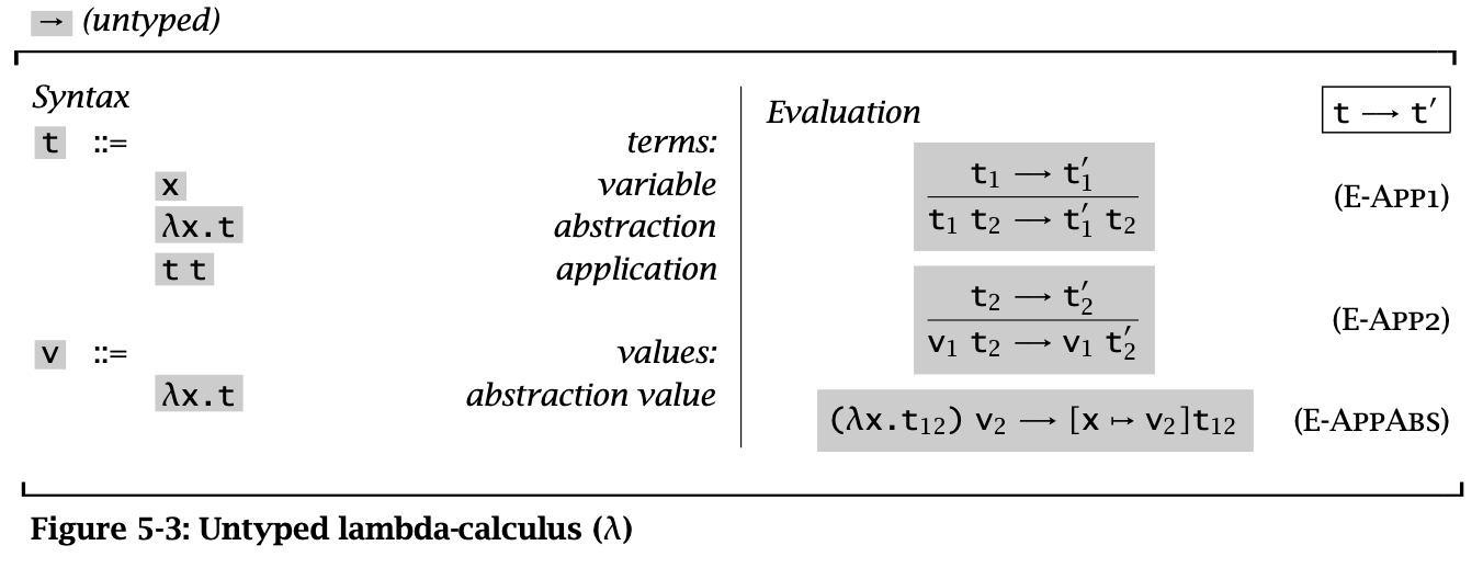
Figure 1: Untyped lambda-calculus
Untyped lambda-calculus 的 evaluation 有两类规则:
E-App1、E-App2:the congruence rulesE-AppAbs:the computation rules
这个规则仅仅是对 call by values 使用的。观察 evaluation relations 可以发现,一般先用 E-App1 化简 \(t_1\),接着用 E-App2 化简 \(t_2\),最后使用 E-AppAbs 进行 reduce。
由于 pure lambda calculus 中的 values 只有 lambda abstractions,所以化简得到的结果一定也是 lambda abstractions。
Rules for other evaluation strategies
full beta-reduction
\[ \dfrac{t_1 \rightarrow t_1’}{t_1\ t_2 \rightarrow t_1’\ t_2} \tag{E-App1} \]
\[ \dfrac{t_2 \rightarrow t_2’}{t_1\ t_2 \rightarrow t_1\ t_2’} \tag{E-App1} \]
\[ (\lambda x. t_{12})\ t_2 \rightarrow [x \mapsto t_2] t_{12} \tag{E-AppAbs} \]
注意这里没有用到
value
normal-order strategy
\[ \dfrac{\operatorname{\mathrm{na}}_1 \rightarrow \operatorname{\mathrm{na}}_1’}{\operatorname{\mathrm{na}}_1\ t_2 \rightarrow \operatorname{\mathrm{na}}_1’\ t_2} \tag{E-App1} \]
\[ \dfrac{t_2 \rightarrow t_2’}{\operatorname{\mathrm{nanf}}_1\ t_2 \rightarrow \operatorname{\mathrm{nanf}}_1\ t_2’} \tag{E-App2} \]
\[ \dfrac{t_1 \rightarrow t_1’}{\lambda x.t_1 \rightarrow \lambda x.t_1’} \tag{E-Abs} \]
\[ (\lambda x. t_{12})\ t_2 \rightarrow [x \mapsto t_2] t_{12} \tag{E-AppAbs} \]
其中用到的三种 term 定义如下:
\begin{aligned} \operatorname{\mathrm{nf}} \Coloneqq && (\text{normal forms}) \\ & \lambda x.\operatorname{\mathrm{nf}} \\ & \operatorname{\mathrm{nanf}} \\ \operatorname{\mathrm{nanf}} \Coloneqq && (\text{non-abstraction normal forms}) \\ & x \\ & \operatorname{\mathrm{nanf}}\ \operatorname{\mathrm{nf}} \\ \operatorname{\mathrm{na}} \Coloneqq && (\text{non-abstraction}) \\ & x \\ & t_1\ t_2 \\ \end{aligned}
dynamic-scoping
Dynamic-scoping 需要在运行期进行替换,因此需要在 contexts(\(\Gamma\))中记录变量对应的值:
\begin{aligned} \operatorname{\mathrm{v}} \Coloneqq && (\text{values}) \\ & \lambda x. e \end{aligned}
\begin{aligned} \Gamma \Coloneqq && (\text{contexts}) \\ & \emptyset \\ & \Gamma, x = t \end{aligned}
\[\dfrac{x = t \in \Gamma}{\Gamma \vdash x \rightarrow t} \tag{D-Var}\]
\[\dfrac{e_{\operatorname{\mathrm{body}}} \rightarrow e_{\operatorname{\mathrm{body}}}’}{e_{\operatorname{\mathrm{body}}}\ e_{\operatorname{\mathrm{arg}}} \rightarrow e_{\operatorname{\mathrm{body}}}’\ e_{\operatorname{\mathrm{arg}}}} \tag{D-App-Lam}\]
\[\dfrac{\Gamma, x = e_{\operatorname{\mathrm{arg}}} \vdash e_{\operatorname{\mathrm{body}}} \rightarrow e_{\operatorname{\mathrm{body}}}’}{\Gamma \vdash (\lambda x. e_{\operatorname{\mathrm{body}}})\ e_{\operatorname{\mathrm{arg}}} \rightarrow (\lambda x. e_{\operatorname{\mathrm{body}}}’)\ e_{\operatorname{\mathrm{arg}}}} \tag{D-App-Body}\]
\[\dfrac{}{\Gamma \vdash (\lambda x. v_{\operatorname{\mathrm{body}}})\ e_{\operatorname{\mathrm{arg}}} \rightarrow v_{\operatorname{\mathrm{body}}}} \tag{D-App-Done}\]
这里的关键在于
D-App-Body,它在运行时会将参数加入到 runtime contexts 中,然后对 body 进行 reduce;完成后使用D-App-Done去掉参数。
lazy strategy
和 call by name 几乎完全一样,但是是 lazy 的。
\[ \dfrac{t_1 \rightarrow t_1’}{t_1\ t_2 \rightarrow t_1’\ t_2} \tag{E-App1} \]
\[ (\lambda x. t_{12})\ t_2 \rightarrow [x \mapsto t_2] t_{12} \tag{E-AppAbs} \]
Big-step style relations
\[ \lambda x. t \Downarrow \lambda x.t \tag{B-Value} \]
\[ \dfrac{ t_1 \Downarrow \lambda x. t_{12} \qquad t_2 \Downarrow v_2 \qquad [x \mapsto v_2] t_{12} \Downarrow v } { t_1\ t_2 \Downarrow v } \tag{B-AppAbs} \]